Introduction to Text Analysis
So far we have started to consider how our potential questions might shape how we work with our data, but today we will be exploring some of the ways in which digital humanists analyze data, especially textual data. Exploring these methods will help us to think about how we might approach our own data and what kinds of questions we might ask of it, as well as the limitations of this kind of analysis.
Final Data Visualization Solutions
Last week I shared a dataset that contained all the counts of the DH tools mentioned in the abstracts from the Index of the DH conference, along with the counts we already had from class and from the original blog post. While optional, one of our assignments was to create a data visualization that would help us to understand the differences between these datasets.
Below are a few of my attempts:
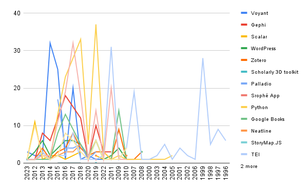
First, I started with Raw Graphs and made a few line graphs, using the following columns:
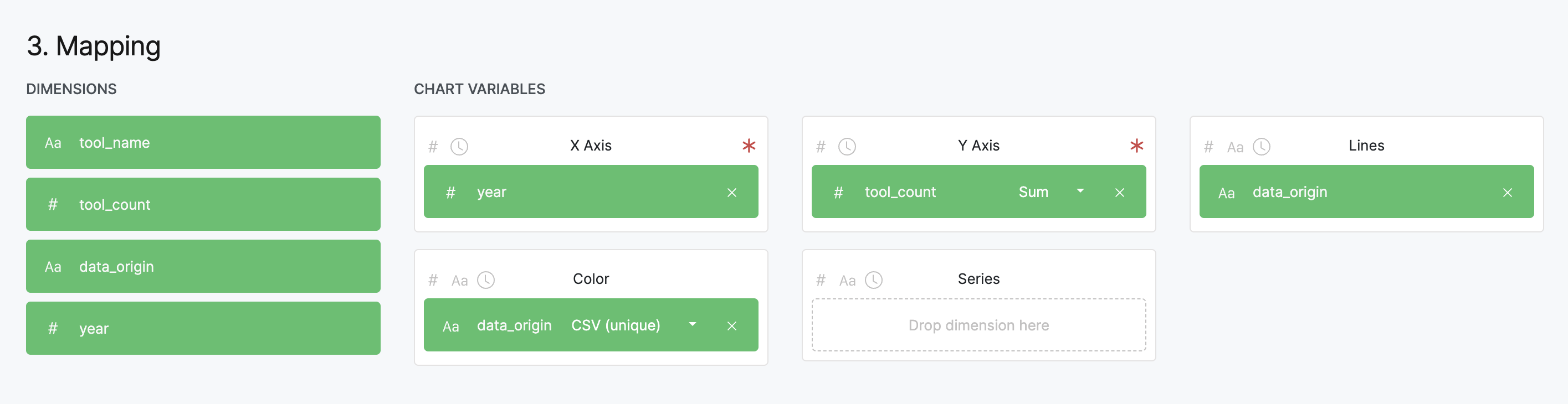
This is what the line graph looks like:
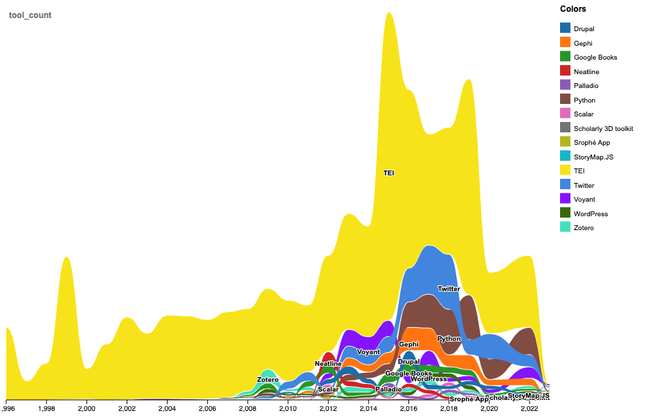
And also used a similar approach to get at the distribution from each of our data origins:
These graphs help demonstrate both the unevenness of our data and the distribution of tools, but there was a few issues with incorrect formatting of dates and difficulty parsing this amount of data. So, I also tried working with Google Sheets.
First, I made a pie chart of all the tools:
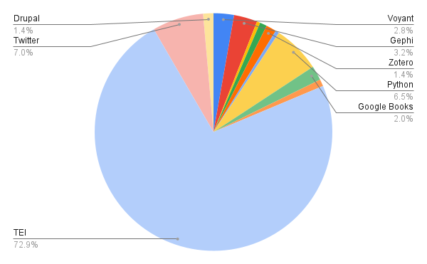
This was helpful in showing the sheer dominance of TEI, but didn’t really help visualize the change over time.
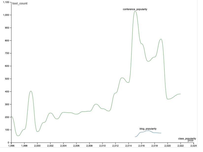
To get at that change though, I had to once again transpose my data since Google Sheets wanted each of the tools as a column to visualize lines. Using OpenRefine, I was able to quickly transform the dataset to look like the following:
Which then allowed me to create a line graph that showed the change over time:
These again were helpful for getting at the change, but Google Sheets did even e with the dates than Raw Graphs did. So, I decided to try DataWrapper.
The first two graphs chart the popularity of tools over time, and I added some annotations to help explain the changes:
These two charts are substantial improvements over the existing ones. The interactivity allows users to hover over to see totals and the annotations help clarify important events. However, there remain a few issues. First, the use of area charts gives the impression that our temporal data is continuous but we are actually missing a few years. Because of that gap, the charts are also a bit misleading. Second, the charts are a bit cluttered and it is difficult to see the trends of individual tools.
To help clarify these trends, I decided to instead create bar charts:
From these two charts we can start to more clearly see the differences between these datasets. For example, the Index of DH Conferences seems to overwhelmingly chart the dominance of TEI, though we can also see that both datasets indicate the growing popularity of Python, and the rise and fall of Twitter. We can further explore the relationships between these datasets if we manipulate them further. So, once again I transposed the original data, this time by data_origin in OpenRefine to create the following dataset:
Organizing the data in this structure allowed me to create a scatter plot that compares the popularity of tools from the Index of DH Abstracts to the blog post, and also compares the popularity of tools from our class to the Index of DH Abstracts:
Both of these charts hint at some interesting outliers, but it is difficult to tell with the dominance of TEI, so I tried removing TEI from the dataset:
Now we can see more clearly that there is a positive relationship (or correlation) between tools mentioned in the Index of DH Conferences and the blog post dataset, and a linear or flat relationship between the Index of DH Conferences and our class dataset. These findings make sense since the blog post was derived from these abstracts and most of the tools in our class dataset only had a value of 1, making it hard to see much of a trend.
You’ll hopefully have noticed by now that two of the tools in our legend (Voyant and StoryMaps) are repeated twice. This repetition is caused by the fact that in the blog post dataset Voyant is listed as Voyant Tools and in the class dataset it is listed as Voyant. Similarly, StoryMaps is listed as StoryMapsJS in the blog post dataset and StoryMaps.JS in the class dataset. You’ll also notice that the blog dataset for some reason does not rank TEI as highly as our conference dataset. All these issues are ones that are symptomatic of the difficulties of analyzing and working with text data.
Text Analysis
The act of trying to count word frequencies is one part of a larger practice called text analysis. Text analysis is a broad term that encompasses a wide range of practices and methods, but at its core it is the practice of trying to understand and analyze texts using computational methods.


Counting words might seem easy at the outset, but actually requires a number of interpretative steps and can be quite useful. For example, Google Ngram Viewer is a popular tool for visualizing word frequencies in the entirety of the Google Books corpus.
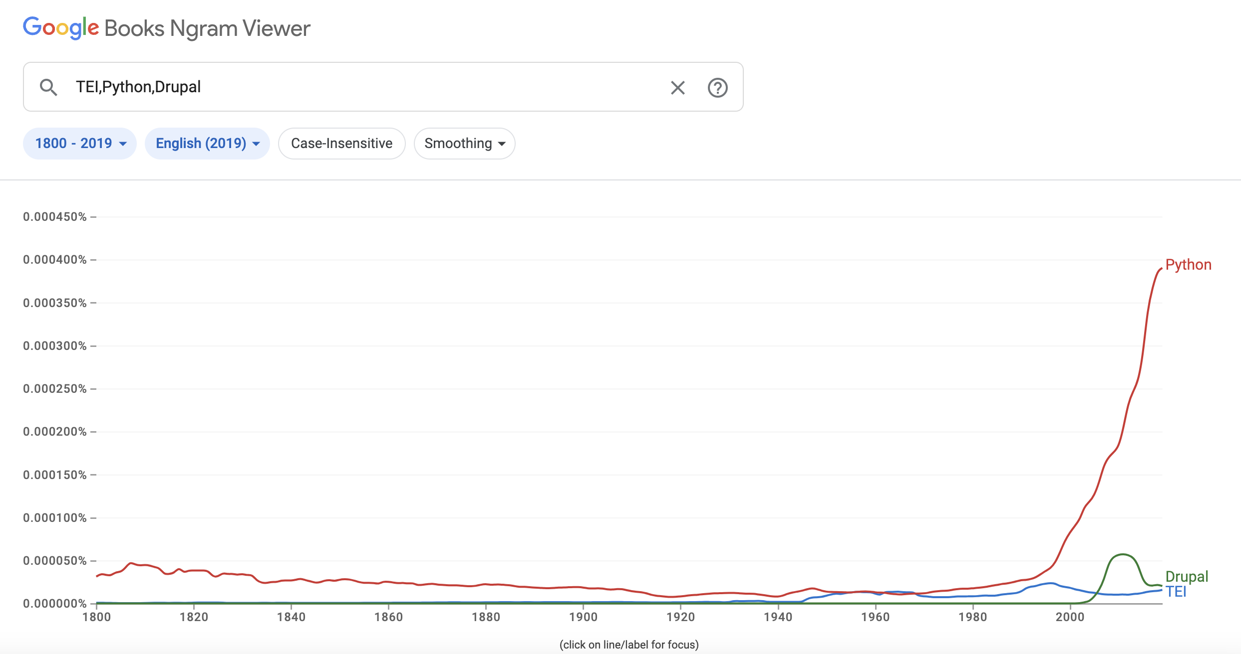
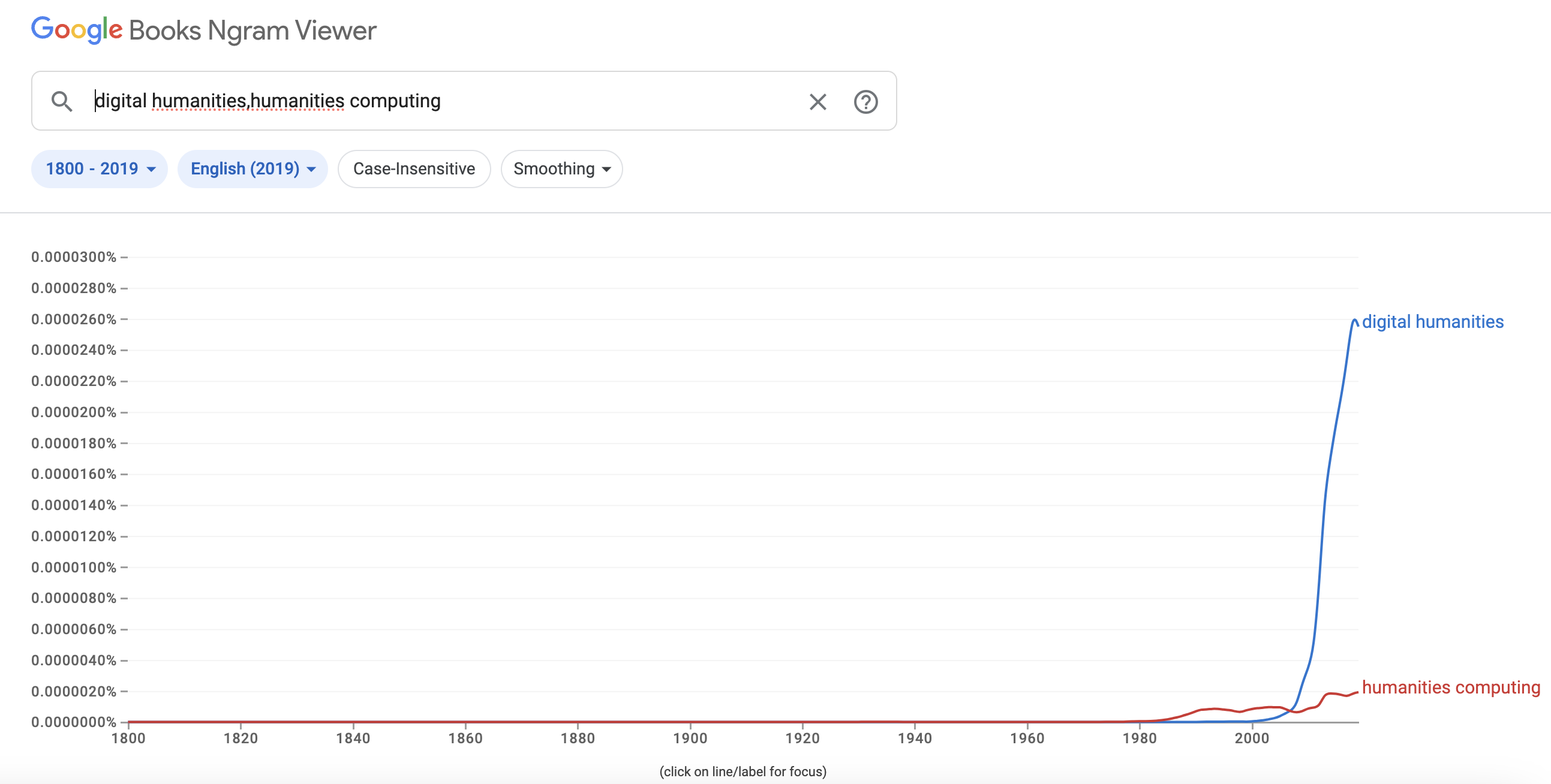
Such figures can seem deceptively obvious but as we have seen with our tools, there can be a number of errors and discrepancies that such graphs can obscure. Indeed, Benjamin Schmidt (whose blog post is one of the curated readings this week) has written extensively about the problems with Google Ngram Viewer and other text analysis tools. For example, he published a critique of a paper that relied on Google Ngram to study whether societies were collectively become more or less depressed over time. The paper’s authors analyzed the Google Books corpus (in English, Spanish, and German languages) spanning over a century to identify “markers of cognitive distortions” such as 2-grams like “everyone thinks” and 3-grams like “I am a”. Schmidt rightfuly pointed out that the authors misunderstood the underlying data and that the Google Books corpus is not a random sample of books, but rather a biased sample of books that are more likely to be popular and thus more likely to be fiction. He also pointed out that the authors did not account for the fact that the corpus is growing over time, and that the authors did not account for the fact that the corpus is not evenly distributed across time. You can read the original critique here Schmidt, Benjamin, Steven T. Piantadosi, and Kyle Mahowald. “Uncontrolled Corpus Composition Drives an Apparent Surge in Cognitive Distortions.” Proceedings of the National Academy of Sciences 118, no. 45 (November 9, 2021): e2115010118. https://doi.org/10.1073/pnas.2115010118 or a helpful summary of the issues here Feigenbaum, James. “Friends Don’t Let Friends Use Google NGrams.” Broadstreet, August 11, 2021. https://broadstreet.blog/2021/08/11/bad-ngrams/.
In the case of our tool frequency dataset, it does not share identical issues but we have already seen some discrepancies around tool counts and names that shares some similarities with our readings that discussed data cleaning and controlled vocabularies. Also part of the issue is that I simply gave you the dataset, without discussing how I created it.
To create the dataset, I wrote some code in Python since counting words is difficult to do in Excel or Google Sheets. The code is available in the following Google Colab notebook for those interested. One of the issues with counting words is that as I’ve said previously, computers are very literal and so while a human might realize that Voyant and Voyant Tools are identical, a computer will not.
So, how would our results look different if we combined these values and also what is the benefit/tradeoffs of normalizing this data?
These graphs show how we can get slightly different results depending on a) which dataset we use and b) the way we count words. The first graph shows the results for counting the term Voyant Tools and we can see that we have four different approaches:
tokenized_countstokenized_lower_countsstring_matching_countsblog_dataset_counts
The last one is the totals from the blog dataset and shows that how those authors generated their data differs from the results I produced using these other methods.
string_matching_counts is what I used in the initial dataset and means I just searched across the entirety of the abstract text for either Voyant or Voyant Tools. This approach means that if someone used the term Voyant whether plural or with an apostrophe or withing another word, I would still count that as part of the term. Such an approach is very expansive and we cans see that it results in the highest counts.
tokenized_counts is a bit more specific and means that I first split the abstract text into individual words and then counted the number of times Voyant or Voyant Tools appeared. This approach means that I would not count Voyant if it was part of another word, but I would still count Voyant Tools if it was plural or had an apostrophe. This approach is a bit more specific.
Finally, tokenized_lower_counts means that I once again split the abstract text into individual words and then counted the number of times Voyant or Voyant Tools appeared, but I also made sure to lowercase all the words before counting them. Remember, computers are dumb so uppercasing and capitalization would indicate a different word. In this case, lowercasing means that I get the most number of terms but again only if it is a separate word.
Normalizing Text
Tokenization was somewhat mentioned in our readings this week when the authors referred to bags of words. Bag of words might sound strange, but it essentially counting words in a text. Like in the example below:
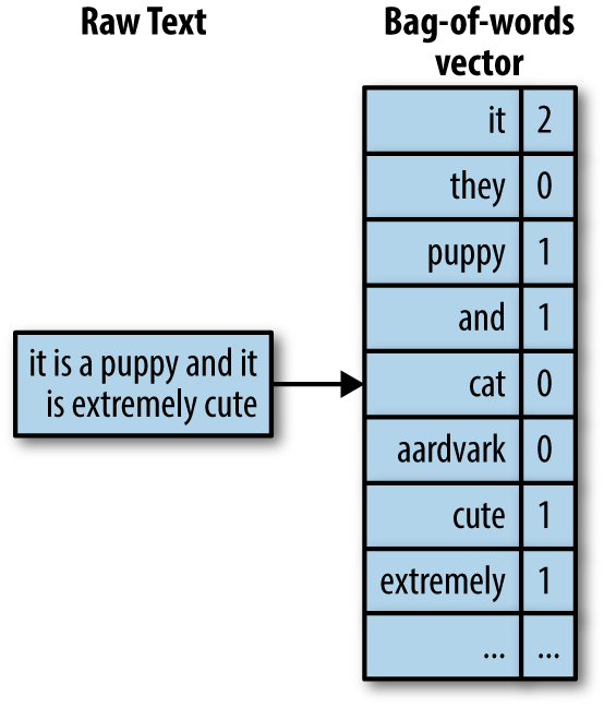
In this instance, the raw text is transformed into a bag of words by removing punctuation and capitalization, followed by counting the words. This is a very simple example, but it is a good way to think about how computers are working with text. This type of process undergirds everything from search engines to spam filters to predictive text.
The first step in this transformation is tokenizing our text, which involves deciding how to split it into individual pieces or features.
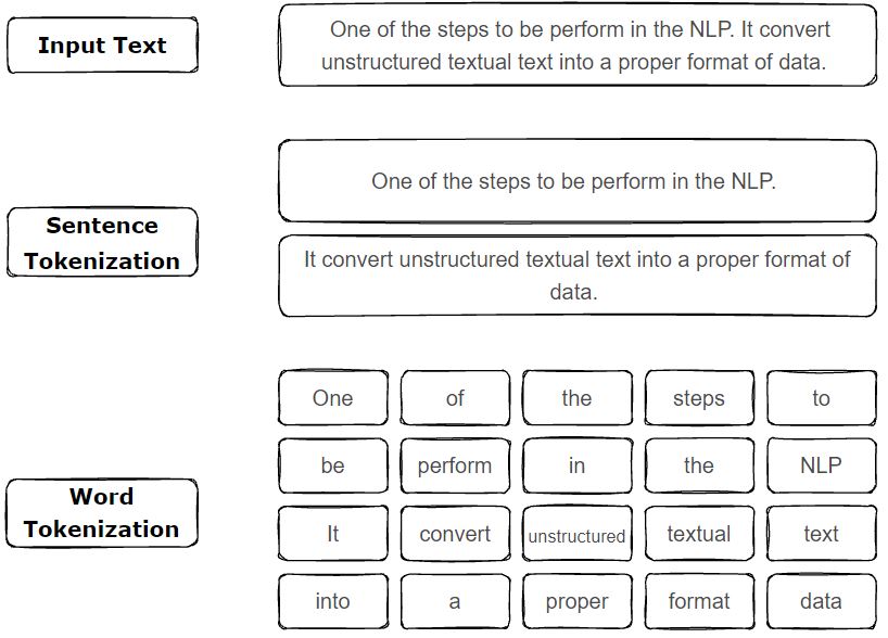
There are a number of ways to tokenize texts, but the most common is to split the text into words. However, this can be a bit tricky since there are a number of ways to split words depending on language and goals. For example, there are processes called lemmatization and stemming that can be used to reduce words to their root form. For example, the words running, runs, and ran can all be reduced to the root word run. This process can be helpful for reducing the number of words in a text, but it can also be problematic since it can also reduce the meaning of a word. For example, the word run can mean a number of different things depending on the context.
Deciding how to clean our textual data, just like visualizing it, requires clarifying our goals and considering many of the topics we have discussed, from how much do we care about privileging algorithmic power to how much do we care about the original context of the text.
Advanced Text Analysis
While our primary focus has been on word counts, our readings this week have shown that text analysis can be much more expansive. In particular, it can help us start to uncover latent meanings across a set of documents or find patterns across a corpora.
Text Analysis with Voyant Tools
As we’ve identified, one of the most popular tools in DH for doing this type of text analysis is Voyant Tools, a tool created by Stéfan Sinclair and Geoffrey Rockwell. Voyant Tools is a web-based tool that allows users to upload their own texts or use texts from the web to analyze. It also allows users to create their own custom tools and visualizations.
Let’s try it out with our Index of DH Abstracts. If you go to either our GitHub repo or Google Drive folder, you’ll find that I’ve created a number of corpora based around our DH Tools. Today, we’ll initially be using the voyant corpora.
Within the folder, you’ll find a csv file that contains the rows from our Index of DH Conferences dataset, and then a folder called voyant. This contains the data we need for Voyant Tools. If you open the folder, you’ll see a number of files that end in .txt. These are the abstracts from the Index of DH Conferences.
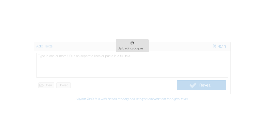
Once we have uploaded that folder, we see the following interface:
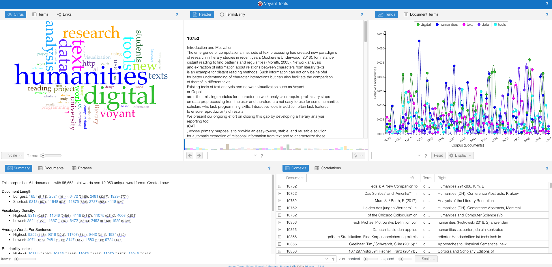
This is pretty overwhelming but there’s an overview of some of the more helpful features:
- Terms: Displays the frequency of individual words. It includes a “sparkline” to show the trend of the term’s frequency over time.
- Documents: Lists the documents in the corpus with quick statistics for each, such as word count and percentage of the total corpus.
- TermsBerry: Visualizes words in the corpus with bubbles sized according to frequency. The proximity and color of the bubbles provide insights into term relationships.
- Trends: Graphs the frequency of individual terms across the entire corpus.
- Keywords in Context: Provides context for any selected term, showing how it’s used within the text.
- The interface allows users to swap tools, configure options for each tool, and access helpful documentation.
We can also explore the extensive documentation for the tool https://voyant-tools.org/docs/#!/guide/about.
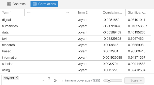
But before we try any of these features, let’s consider what we are analyzing. This corpora contains every abstract that mentioned the tool Voyant. Therefore, with Voyant tools, we can start to explore the differing contexts in which voyant is used in these abstracts (very meta I know!).
To get at these differences, we might use the Correlations tab to see what words most often appear with voyant:
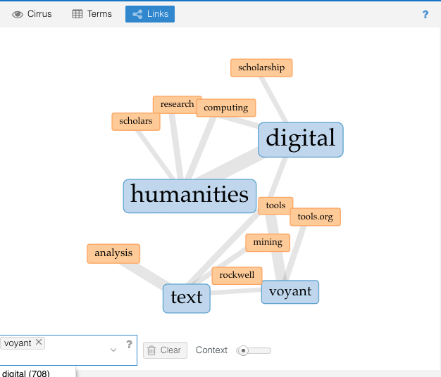
Or we might use the Links tab to see what words are most often connected with voyant:
Or we might even run topic modeling through Voyant and see how voyant is used in different contexts:
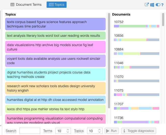
Now that we have these topics, we might return to the initial keywords in the dataset to see how they compare or start comparing voyant to other tools.
In Class Assignment
Working in small groups, start experimenting with Voyant Tools and the various corpora (again available at either our GitHub repo or Google Drive folder). Try to answer the following questions:
- How does the context of various tools change across the corpora? Are there any patterns that might be useful for understanding how these tools are utilized in DH?
- How should this inform our understanding of the tool frequency? Is tool frequency a useful way for studying these abstracts or are there other approaches that might be more useful, like the topics or keywords?
- How might we start updating our keywords or creating a controlled vocabulary based on these findings for DH Tools?
- What are the limitations of this approach? What are the benefits?
In addition to the documentation for Voyant Tools, you might also take a look at Miriam Posner’s tutorial https://github.com/miriamposner/dhvoyant/blob/main/analyze_dh_conference_abstracts_with_voyant.md.
Text Analysis Assignment(s)
Similar to last week, you have the option of two assignments depending on your interests and bandwidth for the week (once again you are welcome to do both if you want). Both assignments should be shared in this GitHub Discussion Forum https://github.com/ZoeLeBlanc/is578-intro-dh/discussions/6 and please specify which assignment you are sharing with your submission.
- Exploratory Meta-Data Analysis: Finding and Assessing Text Analysis in DH
For this assignment, the goal is to find examples of text analysis in DH and trying to identify how the analysis was undertaken and what data was utilized. You can use the examples above or from the readings or find your own. The goal is to try to find at least 1 examples, and then try to identify the following:
- How was the analysis created? What tools were used?
- What does this analysis tell us about not only the data, but trends in DH more broadly?
You are welcome to either create a Markdown file and link to that in the relevant GitHub discussion, or simply post your findings directly in the discussion. If you are having trouble finding examples, please let me know and I can help you with your search.
- Exploratory Text Analysis: Analyzing Texts with DH Tools
For this assignment, the goal is to build from our in-class assignment and undertake more comparisons using text analysis but with additional tools. Your goal is to work with one of the following tools:
- AntConc https://www.laurenceanthony.net/software/antconc/ (requires downloading)
- MALLET https://mimno.github.io/Mallet/topics.html or for a web browser version JSlda https://mimno.infosci.cornell.edu/jsLDA/jslda.html
- WordCounter from DataBasic https://www.databasic.io/en/wordcounter/ (also web browser)
and then compare the results from one of these tools to what you produced in Voyant Tools. You should once again use this data: GitHub repo or Google Drive folder, though if you have an idea for a different corpora you are welcome to use that instead or ask the instructor for help generating one from our Index of DH Abstracts.
In your assignment, you can use the same corpora or a different one from the one you used in class, but the goal is to try to identify the differences between these tools and what they tell us about the data. In terms of sharing results, you should either create a Markdown file or Google Doc that outlines your findings and then link to that in the relevant GitHub discussion. If you are having trouble with the tools, please let me know and I can help you troubleshoot.
Remember this assignment is exploratory so there is no right or wrong answer, but you should try to identify the differences between these tools and what they tell us about the data.